Finally, after enduring 6 gruelling months of blood and sweat combined with another 4 months of waiting, I received the holy news of acceptance today! Ah, it sure felt like a huge weight has been lifted off my shoulder.

Since sharing is caring, and I cannot wait to write about my first research paper, let me give you a short introduction to the world of efficiently mapping streaming heterogeneous data into RDF.

We shall begin with an introduction to the landscape of RDF stream generations.

How does the RDF stream generation workflow look like?

A very simple RDF stream generation workflow as shown in Figure 1 consists of three distinct components:

1. Unbounded heterogeneous data source. This is a data source which could potentially never end so long as the source is healthy. Furthermore, the data format of the source can be arbitrary. An example of such data source would be a 24/7 live temperature sensor.

2. Streaming RDF generator engine. The meat of this blog post, where we contribute a highly efficient mapping engine. The job of this component is to map incoming heterogeneous data into RDF compliant data format such as N-Triples.

3. RDF stream processing engine. Any client engines that consume RDF data streams and process them. An example would be a RDF stream reasoning engine.

In an ideal wonderland, there are no problems in this workflow. Sadly, we live in a reality where Murphy's Law has its little dirty hands in every aspect of our lives. Anything that can go wrong will go wrong, and at the worst possible time .

3 Challenges in stream mapping workflow

So, what are the things that could go wrong ? We could discuss all of them but it will never end until the end of times. Thus, let us focus on the 3 problems or challenges in a stream mapping workflow in the context of this work.

Challenge 1: High velocity input data stream

In a streaming environment, the characteristics of a data stream can be unpredictable from the perspective of the RDF stream generator. You cannot control how the data sources will behave. It is possible that the velocity of the data streams, the number of messages per second, will be very high. This is the first challenge for RDF stream generators; dealing with the high velocity of the data streams.

Challenge 2: Low latency output of generated RDF statements

As the velocity of the data streams increases, so does the processing power required for the RDF stream generator. If the RDF stream generator could not handle the increase data velocity, it pays the price with a high latency in the generated RDF output stream $-$ our second challenge in stream mapping workflow.

Challenge 3: Joining multiple input data stream

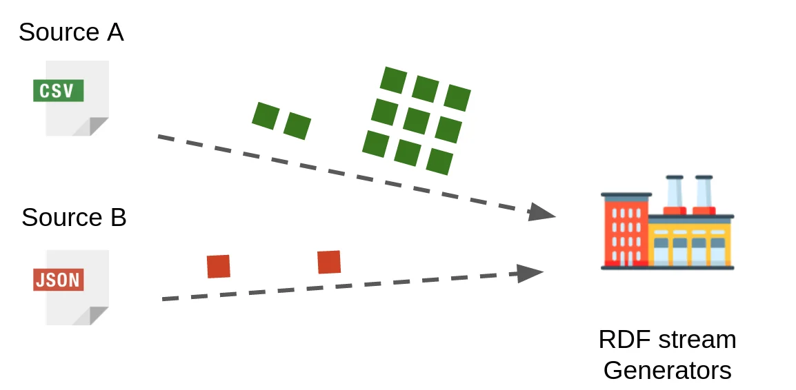
The given scenario in Figure 1, mapping a data stream to RDF, does not enrich the original data. Even if multiple streams are being processed simultaneously by the RDF stream generator, we do not have correlation between different data stream, therefore, there is no data enrichment. A frequent and most utilized method for data stream enrichment is data joins. In traditional relational databases, joins could be implemented with full knowledge of the datasets enabling join optimizations to speed up the process. However, in an unbounded data stream, we do not have the picture of the whole dataset to optimize the data stream joins. This leads us to our third challenge; how do we efficiently handle multiple data stream joins?

RMLStreamer-SISO to the rescue!

We introduce RMLStreamer-SISO! A highly efficient unbounded heterogeneous data streams to RDF stream mapping engine. The engine could scale horizontally (distributed across cluster) and vertically (multithreading). RMLStreamer-SISO processes the unbounded heterogeneous data streams at low latency with high throughput, it has the ability to execute data transformation operators dynamically, and it also joins multiple data streams using dynamic windows. Such performance is achieved by incorporating a dataflow paradigm in our stream mapping architecture. How does such a stream mapping architecture look like?

RMLStreamer-SISO stream mapping architecture

A dataflow paradigm represents the mapping workflow as a directed graph with data flowing between different processing nodes. We modelled RMLStreamer-SISO as a dataflow program consisting of 4 different tasks as shown in Figure 3.

The functionalities of the 4 tasks are listed as follows:

1. Ingestion task: The incoming data from the input data streams are ingested one by one. These records are then individually transformed into an internal abstract data structure and partitioned for parallel processing further down the stream mapping pipeline.

2. Mapping task: Self evident in the name, this task maps the output from ingestion task to RDF statements. The mapping task is stateless and handles the mapping in a streaming manner.

3. Collector task: The generated RDF statements from the mapping task is collected and pushed to sinks such as files, websockets, and Kafka topics.

4. Pre-Mapping task: This is where the data transformations, and the stream joins take place. Both the data transformation, and the stream joins are executed dynamically and on demand. The pre-mapping tasks can be chained after each other; for example, you can apply a data transformation operation first, join the data, and then apply a data transformation operator again before sending the compiled results to the mapping task.

By modularizing the stream mapping architecture in a dataflow model, we could employ distributed stream processing concepts readily. In fact, for our implementation, this architecture was crucial to overcoming 2 of the 3 challenges we described earlier.

Implementation of RMLStreamer-SISO

Before we go into the techniques employed to overcome the challenges, we'll give a brief introduction into the implementation of RMLStreamer-SISO.

We implemented RMLStreamer-SISO on top of a stream processing framework, Apache Flink. This enables us to enjoy all the benefits brought by Apache Flink out-of-the-box; ability to scale vertically and horizontally on demand, and the failure recovery in case the mapping process gets interrupted. Moreover, due to the modular architecture, the different modular tasks could be adapted and mapped to Flink operators allowing us enjoy the dynamic scaling of Apache Flink. For example, if the mapping task could not keep up with the ingestion rate of the ingestion task, Flink will scale the mapping task automatically in order to reduce the back pressure and ensure low latency, and high throughput generation of RDF statements.

Challenge mitigation strategies

Two challenges are tackled by our modular architecture through the exploitation of the underlying Apache Flink framework:

1. High velocity input data streams.

2. Low latency generation of RDF statements streams from heterogeneous data streams.

What about the third one? How do we handle joining multiple input data streams which are unbounded? We cannot keep track of the whole data stream in memory, it is impossible! We need a partial view of the unbounded data stream: a window. In order to show how a window join works on a data stream, I like to use what I call a fixed size bus problem.

Fixed size bus analogy

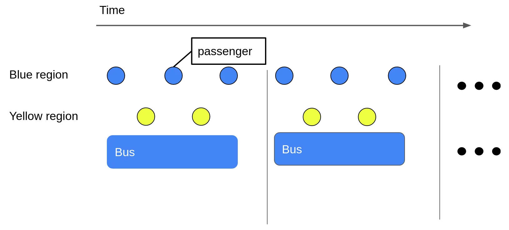
In a fixed size bus scenario, you have passengers from two regions at the bus stop: blue and yellow region. These passengers arrive at the bus stop and board the first available bus. The bus leaves the stop at a fixed interval at which point they will process the info of the passengers to find common infos between the two regions (a join). Ideally, the processing will be executed efficiently with sufficient data output; however, the reality of the data stream environment is not so simple. The characteristics of a data stream can change over time.

The problems

Imagine the arrival rate of the passengers changes over time, the fixed size bus will encounter two problems: inefficient memory usage and high latency.

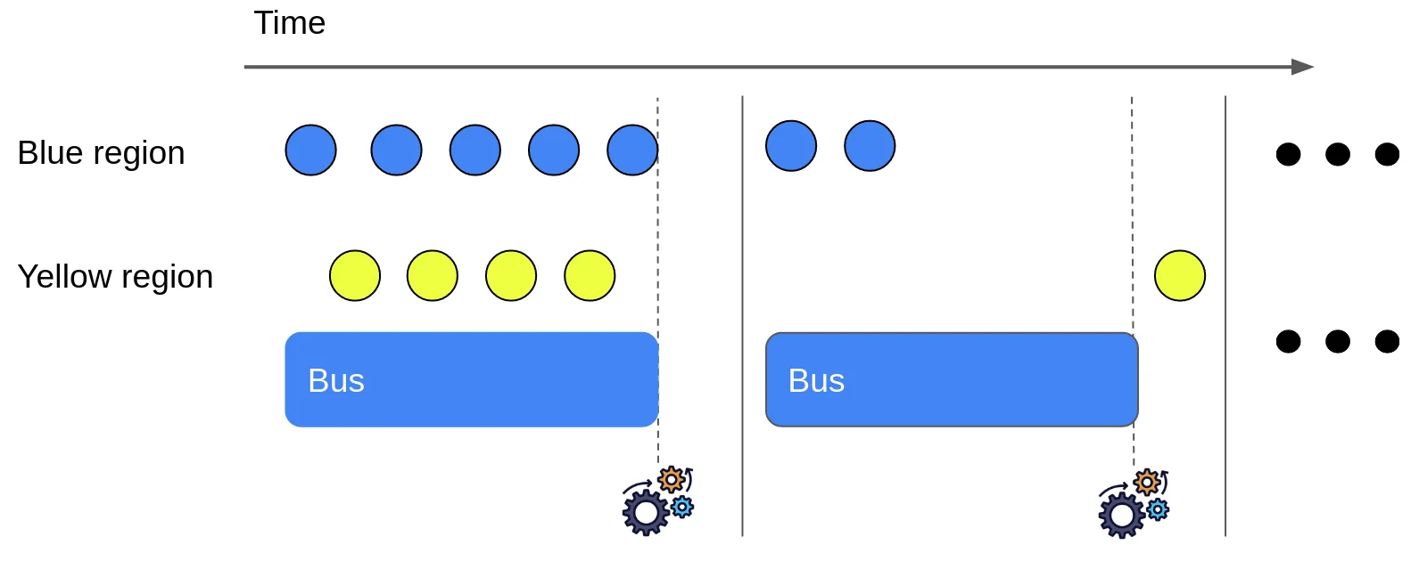
Fixed size bus suffers from inefficient memory usage because of the amount of passengers the bus has to keep track. In the first sub scenario in Figure 5, the high arrival rate of the bus causes it to remember those passengers for info processing when it departs. This increase in the amount of passengers leads to an increase in latency due to having more work for data processing. On the other hand, when the arrival rate of passengers changes over time and lowers, we land ourselves in the situation of the second sub scenario. The fixed size bus is just not big enough to contain the one late passenger from yellow region, leading to no output being produced when the bus departs the stop; remember, we are trying to find common infos between the two regions, therefore at least one passenger from each region needs to be inside the bus. Thus, we have a few problems with fixed size buses: high memory usage, high latency, low throughput, and inefficient memory usage when enough of them is available.

The solution: dynamic size vehicles

To solve the aforementioned problems with fixed size bus, we introduce a dynamic sizing solution.

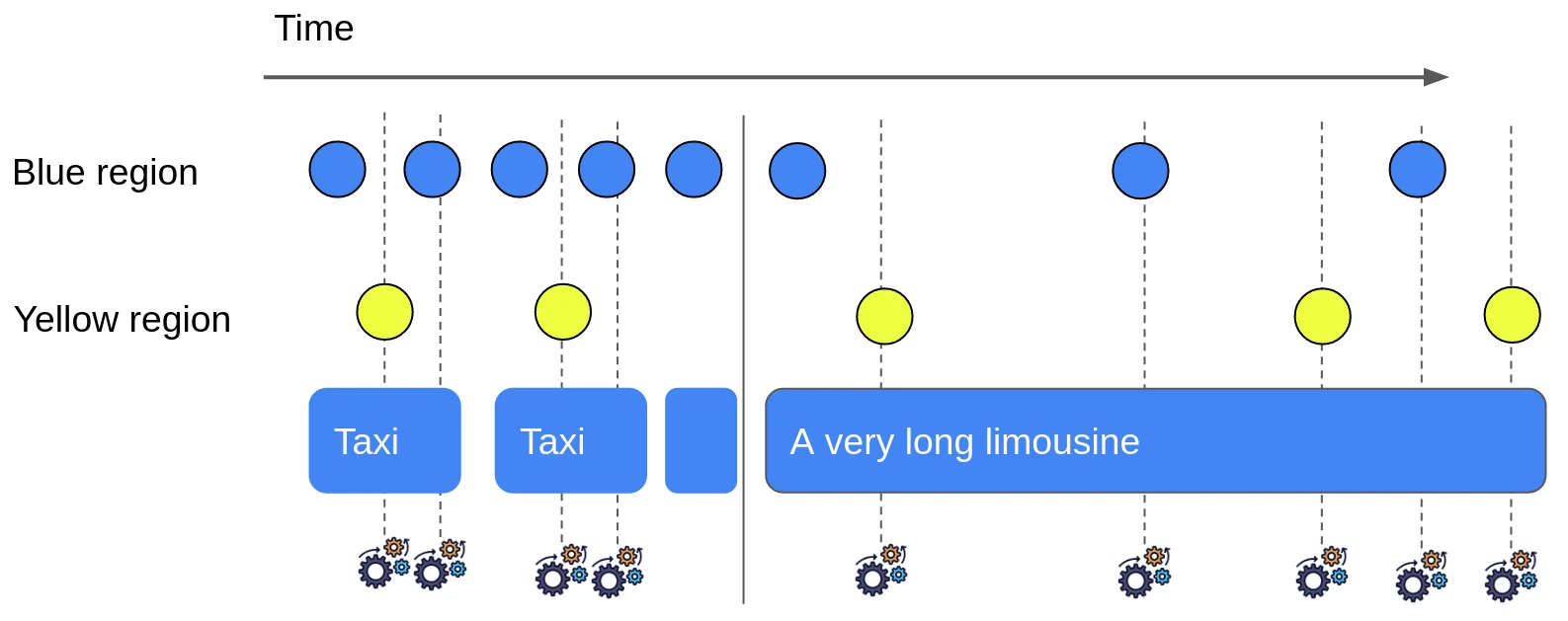
When the arrival rate of the passengers is high, we will use Taxi's of smaller size to ensure that the memory usage is kept low. Similarly, we will deploy long limousine to wait for more passengers when the arrival rate of the passengers drop. This ensures that the memory usage is low during high arrival rate. At the same time, the long limousine use the memory efficiently to its fullest when the arrival rate is low. With this, dynamic size vehicles offers low, and efficient memory usage.

To tackle the high latency, and low throughput, dynamic window will execute eager processing instead of waiting for the vehicle to leave. We will process the current passenger inside the vehicle as soon as possible (indicated by the cogwheels at different passenger arriving). We do not wait for all passengers to arrive first, increasing the throughput of the results generated.

Performance of RMLStreamer-SISO

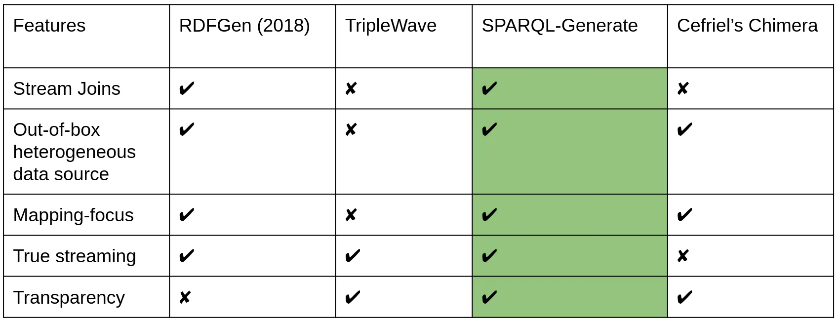
In order to evaluate the RMLStreamer-SISO, we compiled a set of features to choose the best candidate to evaluate RMLStreamer-SISO against. Table 1 shows that SPARQL-Generate has the most common set of features with RMLStreamer-SISO to be evaluated against. The other SOTAs are not considered since they do not fulfil our requirement for evaluation.

TripleWave

TripleWave¹ requires a custom implementation to process each data stream and feed it in TripleWave, which means it cannot be used as it is. Moreover, TripleWave is meant purely for feeding RDF streams to RDF stream processing engines without performing joins, therefore it would have been an unfair comparison both in terms of features and scope.

Cefriel's Chimera

Cefriel's Chimera² restarts the RDF mapping engine with every data record, which means that the processing of the input and mapping is not performed in a true streaming manner; the comparison would not be meaningful.

RDF-Gen (2018)

Finally, although RDF-Gen (2018) ³ fulfils almost all the feature sets, it lacks transparency. We could not verify the implementation since it is closed source and there is a lack of instruction to run the engine. Therefore, it cannot be considered for evaluation.

Benchmark setup

The setup of our benchmark consists of two crucial parts: 1) the benchmark architecture and 2) the workloads design.

Architecture

One aspect often overlooked when conducting a benchmark is resource contention between the benchmark system, and the system under test (SUT). If no isolation is taken care of during the benchmark, the non-SUT components in the benchmark will have significant influence on the performance measurement of SUT. For example, I/O operations of the non-SUT components can cause the SUT's I/O operations to degrade in performance leading to negative performance showing up in measurements.

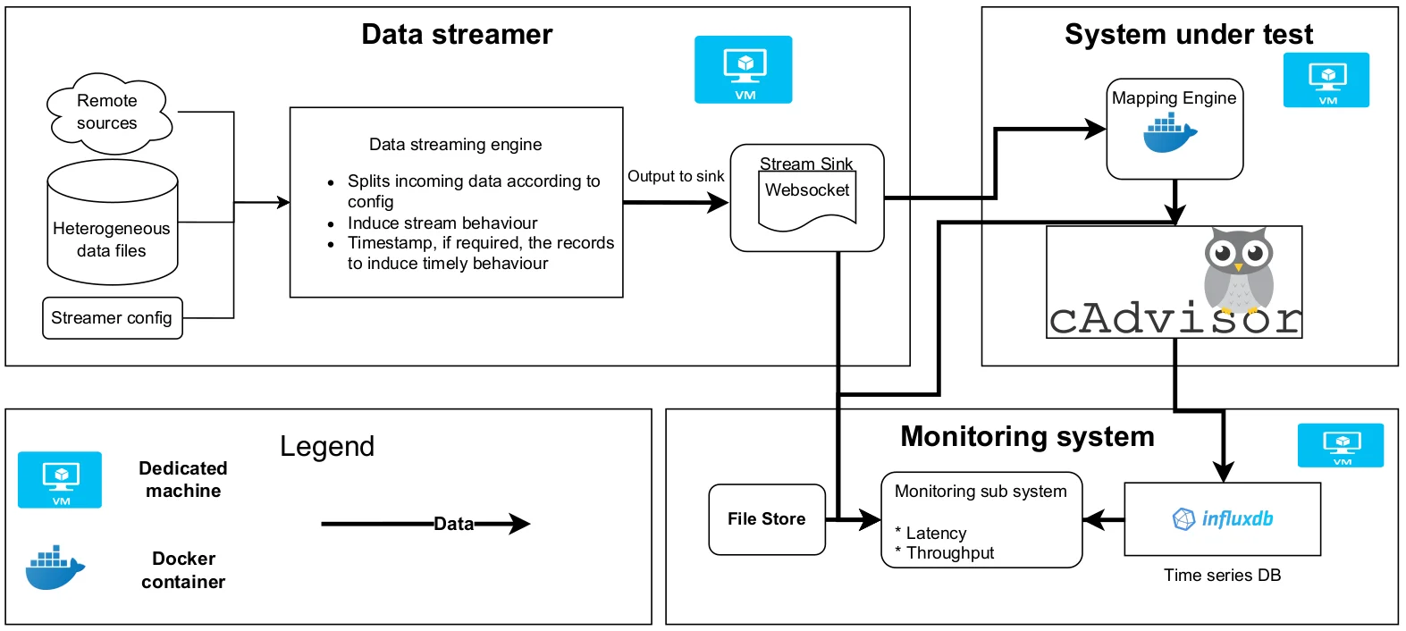
We proposed a modular benchmark architecture for our benchmark as shown in Figure 7. The architecture is a modification of RSPLab with a custom data stream component. We treat the SUTs as a blackbox to ensure that the measurement of the metrics incurs no performance penalty nor resource contention with the SUTs.

Workload designs

We designed three workloads for the benchmark:

1. Constant Workload: Evaluates the mapping engines ability to cope with increasing velocity of data stream. Throughput and latencies are the main metrics to be measured here.

2. Periodic Workload: This workload evaluates the mapping engines' capability to adapt to the dynamic streaming environment. A burst of data records is emitted periodically to simulate hot period of traffic.

3. Scalability Workload: This workload evaluates the scalability of join operations on multiple input data streams as the velocity of the data stream increases.

Workload metrics

For the metrics, we measured the following statistics prevalent in benchmark of stream processing engines:

1. Throughput of the engine (msg/s): We measured the throughput of the engine to measure the rate at which RDF statements are generated.

2. Event time latency (ms): Event time latency is considered instead of processing time latency to also include the effect of coordinated occlusion, the queueing time of the data inside the processing engine.

3. CPU usage (%): Checks how efficient the stream processing engine uses the available CPU resources.

4. Memory usage (GB): Checks memory usage efficiency of the stream processing engine.

RMLStreamer-SISO performs efficiently under increasing velocity

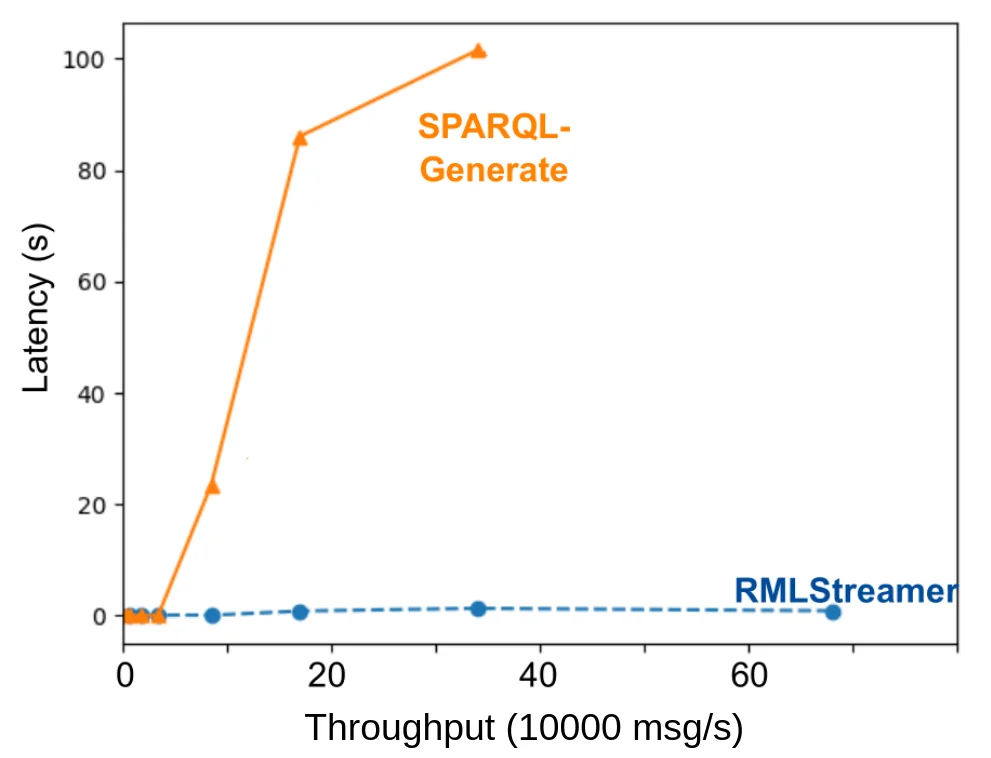
Figure 8 shows even with increasing throughput, RMLStreamer-SISO outperforms SPARQL-Generate by a huge margin in terms of latency. It consistently maintains sub second latency throughout the experiment with increasing input velocity at each run. SPARQL-Generate on the other hand, is shown to be unsustainable once the input velocity is higher than 10,000 msg/s. The latency increased logarithmically until 100s.

Handles huge dynamic data bursts too

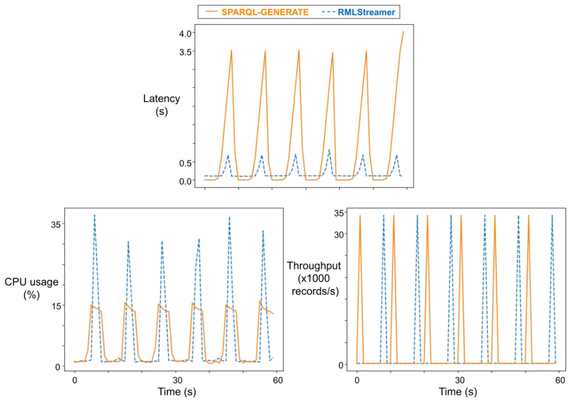
The periodic burst workload measures the adaptability of the engine to the recurring burst of data stream. Last minute of the evaluation is measured to ensure the engines are stable without warm-up overhead. Two graphs of interest for analysis here; the latency, and the CPU usage graphs. For the latency graph, the spike of the RMLStreamer-SISO's latency
is significantly handling the burst of data; whereas SPARQL-Generate's latency spiked around 3.5s. Although RMLStreamer-SISO uses more CPU resource than SPARQL-Generate; The CPU usage graph shows that the spike of RMLStreamer-SISO is narrower than the spike of SPARQL-Generate. RMLStreamer-SISO uses CPU efficiently and for a shorter period than SPARQL-Generate to handle the burst of data: showing that it adapts to the periodic data bursts well.

Scalability of RMLStreamer-SISO in handling multiple stream joins

Metrics	Unparallelized mode	Parallelized mode
Median latency	50000ms	57ms
Minimum latency	13653ms	8ms

Scalability wise, we showed that RMLStreamer-SISO scales exceptionally well to ensure low latency joining of multiple data stream and mapping heterogeneous data to RDF (Table 2). Parallelized mode of RMLStreamer-SISO has sub 100ms latency while the minimum latency of unparallelized mode is more than 10s. This shows that parallelizing through distribution of workload significantly benefits the stream processing engine.

Conclusion

RMLStreamer-SISO shows great promises in mapping unbounded heterogeneous data stream to RDF stream. It could be incorporated into existing workflow to generate high quality RDF data. RMLStreamer-SISO increases the availability of RDF streams following the high availability of data streams. Using a low-latency tool like RMLStreamer- SISO, legacy streaming systems could exploit the unique characteristics of real- life streaming data, while enabling analysts to exploit the semantic reasoning using knowledge graphs in real-time. I believe that the future of RDF generation lies in the domain of stream processing.

Footnotes

1. TripleWave: https://streamreasoning.org/TripleWave/ ↩

2. Cefriel's Chimera: https://github.com/cefriel/chimera ↩

3. RDF-Gen: https://dl.acm.org/doi/10.1145/3227609.3227658 ↩